
An analysis of the Titanic dataset
Published:
An analysis of the Titanic dataset
# Imports

# pandas
import pandas as pd
from pandas import Series,DataFrame

# numpy, matplotlib, seaborn
import numpy as np
import matplotlib.pyplot as plt
import seaborn as sns
sns.set()
sns.set_style('whitegrid')
%matplotlib inline
# get titanic & test csv files as a DataFrame
titanic_df = pd.read_csv("train.csv")
test_df    = pd.read_csv("test.csv")

# preview the data
titanic_df.head()
| PassengerId | Survived | Pclass | Name | Sex | Age | SibSp | Parch | Ticket | Fare | Cabin | Embarked | |
|---|---|---|---|---|---|---|---|---|---|---|---|---|
| 0 | 1 | 0 | 3 | Braund, Mr. Owen Harris | male | 22.0 | 1 | 0 | A/5 21171 | 7.2500 | NaN | S |
| 1 | 2 | 1 | 1 | Cumings, Mrs. John Bradley (Florence Briggs Th... | female | 38.0 | 1 | 0 | PC 17599 | 71.2833 | C85 | C |
| 2 | 3 | 1 | 3 | Heikkinen, Miss. Laina | female | 26.0 | 0 | 0 | STON/O2. 3101282 | 7.9250 | NaN | S |
| 3 | 4 | 1 | 1 | Futrelle, Mrs. Jacques Heath (Lily May Peel) | female | 35.0 | 1 | 0 | 113803 | 53.1000 | C123 | S |
| 4 | 5 | 0 | 3 | Allen, Mr. William Henry | male | 35.0 | 0 | 0 | 373450 | 8.0500 | NaN | S |
Passenger ID, name, and ticket will be dropped. Fare could be other candidate to be dropped (correlation with class), and perhaps cabin too. I’ll initially assume that cabin doesn’t help predict Survive, and let’s first see what happens with fare and class.
train = titanic_df.drop(['PassengerId','Name','Ticket','Cabin'], axis=1)
test    = test_df.drop(['PassengerId','Name','Ticket','Cabin'], axis=1)
#We also add a 1/0 variable for Sex
df_sex=pd.get_dummies(train['Sex'],drop_first=True)
train=train.join(df_sex)

df_sex_2=pd.get_dummies(test['Sex'],drop_first=True)
test=test.join(df_sex_2)
#Also df['Gender'] = df['Sex'].map( {'female': 0, 'male': 1} ).astype(int)


#Dummies for Pclass too

df_pclass=pd.get_dummies(train['Pclass'],prefix='Class').astype(int)
train=train.join(df_pclass)

df_pclass_2=pd.get_dummies(test['Pclass'],prefix='Class').astype(int)
test=test.join(df_pclass_2)
train.head()
| Survived | Pclass | Sex | Age | SibSp | Parch | Fare | Embarked | male | Class_1 | Class_2 | Class_3 | |
|---|---|---|---|---|---|---|---|---|---|---|---|---|
| 0 | 0 | 3 | male | 22.0 | 1 | 0 | 7.2500 | S | 1 | 0 | 0 | 1 |
| 1 | 1 | 1 | female | 38.0 | 1 | 0 | 71.2833 | C | 0 | 1 | 0 | 0 |
| 2 | 1 | 3 | female | 26.0 | 0 | 0 | 7.9250 | S | 0 | 0 | 0 | 1 |
| 3 | 1 | 1 | female | 35.0 | 1 | 0 | 53.1000 | S | 0 | 1 | 0 | 0 |
| 4 | 0 | 3 | male | 35.0 | 0 | 0 | 8.0500 | S | 1 | 0 | 0 | 1 |
#Deal with age

avg_age_train=train['Age'].mean()
std_age_train=train['Age'].std()
nans_age_train=train['Age'].isnull().sum()

avg_age_test=test['Age'].mean()
std_age_test=test['Age'].std()
nans_age_test=test['Age'].isnull().sum()

#Generate random ages
rand_1 = np.random.randint(avg_age_train-std_age_train,avg_age_train+std_age_train,size=nans_age_train)
rand_2 = np.random.randint(avg_age_test-std_age_test,avg_age_test+std_age_test,size=nans_age_test)

#Fill NaNs
#train["Age"][np.isnan(train["Age"])] = rand_1
#test["Age"][np.isnan(test["Age"])] = rand_2
#Median better than mean to avoid outliers
train['Age'].fillna(train['Age'].median(), inplace=True)
test['Age'].fillna(test['Age'].median(), inplace=True)
#Check
np.all(~np.isnan(train["Age"]))
True
corrmat=train[['Survived','Class_1','Class_2','Class_3','SibSp','Parch','Fare','male','Age']].corr()
print(corrmat)
sns.heatmap(corrmat,vmax=.8,annot=True)
          Survived   Class_1   Class_2   Class_3     SibSp     Parch  \
Survived  1.000000  0.285904  0.093349 -0.322308 -0.035322  0.081629
Class_1   0.285904  1.000000 -0.288585 -0.626738 -0.054582 -0.017633
Class_2   0.093349 -0.288585  1.000000 -0.565210 -0.055932 -0.000734
Class_3  -0.322308 -0.626738 -0.565210  1.000000  0.092548  0.015790
SibSp    -0.035322 -0.054582 -0.055932  0.092548  1.000000  0.414838
Parch     0.081629 -0.017633 -0.000734  0.015790  0.414838  1.000000
Fare      0.257307  0.591711 -0.118557 -0.413333  0.159651  0.216225
male     -0.543351 -0.098013 -0.064746  0.137143 -0.114631 -0.245489
Age      -0.064910  0.323896  0.015831 -0.291955 -0.233296 -0.172482

              Fare      male       Age
Survived  0.257307 -0.543351 -0.064910
Class_1   0.591711 -0.098013  0.323896
Class_2  -0.118557 -0.064746  0.015831
Class_3  -0.413333  0.137143 -0.291955
SibSp     0.159651 -0.114631 -0.233296
Parch     0.216225 -0.245489 -0.172482
Fare      1.000000 -0.182333  0.096688
male     -0.182333  1.000000  0.081163
Age       0.096688  0.081163  1.000000


<matplotlib.axes._subplots.AxesSubplot at 0x7f8d623df748>
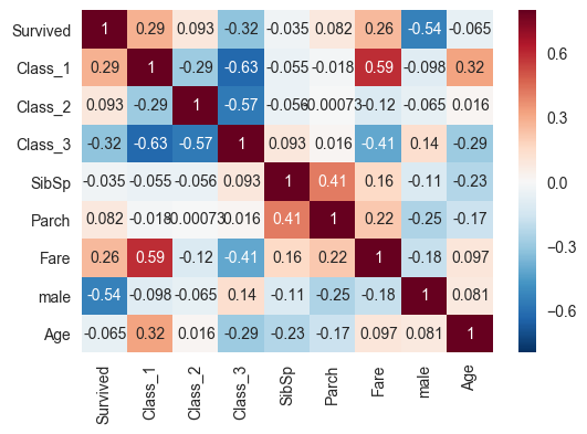
There doesn’t seem to be NaNs or weird things, no need for cleaning. But we do need to fill some values for age. Also, I should check whether embarked does something. Let’s go with that first.
sns.countplot(x="Embarked", data=train);
plt.figure();
sns.barplot(x='Embarked',y="Survived", data=train);
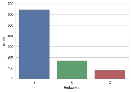
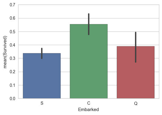
But is this spurious due to higher variability in C and Q because there are less of them? Maybe. Perhaps it’d be worthwhile to keep these around, so let’s dummy them, and run a regression.
It seems to make sense to impute the missing values to S, as it is the most common, and near the average
train['Embarked']=train['Embarked'].fillna('S')
test['Embarked']=test['Embarked'].fillna('S')

df_em=pd.get_dummies(train['Embarked'],prefix='Embarked')
Let’s study the fare-class relationship
# First, I need to extract the fares and  group them by Pclass, then plot.
#pclass_fare=train[['Fare','Pclass']]
#print(pclass_fare.groupby(['Pclass']).describe())
#print(pclass_fare.groupby(['Pclass']).mean())
#sns.boxplot(x="Pclass", y="Fare", data=pclass_fare);
As expected, the correlation seems to be there. But how strong is the correlation?
Hm, perhaps better to keep it. $R^2$ is not that high
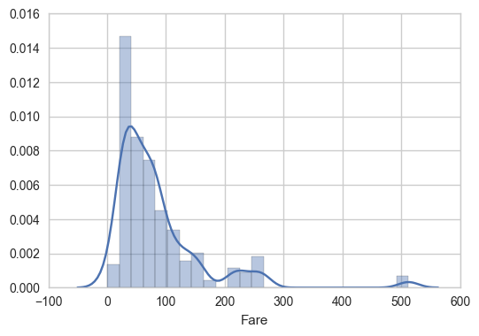
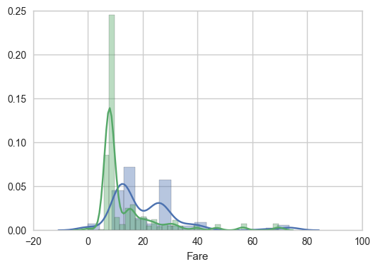
For fun, how are fares by Pclass distributed?
sns.distplot(train[train['Class_1']==1]['Fare'])
plt.figure()
sns.distplot(train[train['Class_2']==1]['Fare'])
sns.distplot(train[train['Class_3']==1]['Fare'])
/home/artir/anaconda3/lib/python3.5/site-packages/statsmodels/nonparametric/kdetools.py:20: VisibleDeprecationWarning: using a non-integer number instead of an integer will result in an error in the future
  y = X[:m/2+1] + np.r_[0,X[m/2+1:],0]*1j


<matplotlib.axes._subplots.AxesSubplot at 0x7f8d415d74e0>
Back to Embarked and survived:
# result = sm.ols(formula="Survived ~Embarked_Q+Embarked_C+Embarked_S ", data=train).fit()
# print(result.params)
# print (result.summary())
#R2 too small, disregard.
So finally, the choosen features will be Pclass, Fare, male, and age. Time to do some predictions.
# define training and testing sets
#There happens to be one missing element in Fare. So let's fix that
test["Fare"].fillna(test["Fare"].median(), inplace=True)
X_train = train[['Pclass','Fare','male','Age']]
Y_train = train[["Survived"]]
X_test  = test[['Pclass','Fare','male','Age']]
# Logistic Regression
# machine learning
from sklearn.linear_model import LogisticRegression
logreg = LogisticRegression()

logreg.fit(X_train, Y_train.values.ravel())

Y_pred = logreg.predict(X_test)
logreg.score(X_train, Y_train)
0.7912457912457912
Let’s add some more features
train['FamilySize'] = train['SibSp'] + train['Parch']
test['FamilySize'] = test['SibSp'] + test['Parch']
# If greater than zero, it'll be one. If not, zero
train['HaveFamily'] = 0
test['HaveFamily'] = 0
test['FamilySize'] = test['SibSp'] + test['Parch']
train['FamilySize'] = train['SibSp'] + train['Parch']
test.loc[test['FamilySize']>0,'HaveFamily']=1
train.loc[train['FamilySize']>0,'HaveFamily']=1
#Childs
train['child'] = 0
test['child'] = 0
test.loc[test['Age']<15,'child']=1
train.loc[train['Age']<15,'child']=1
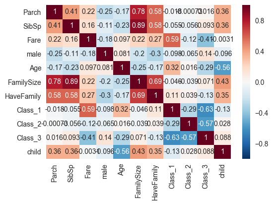
predictors=['Parch','SibSp','Fare','male','Age','FamilySize','HaveFamily','Class_1','Class_2','Class_3','child']
X_train = train[predictors]
Y_train = train[["Survived"]]
X_test = test[predictors]
corrmat=train[predictors].corr()
print(corrmat)

a=sns.heatmap(corrmat,annot=True)
               Parch     SibSp      Fare      male       Age  FamilySize  \
Parch       1.000000  0.414838  0.216225 -0.245489 -0.172482    0.783111
SibSp       0.414838  1.000000  0.159651 -0.114631 -0.233296    0.890712
Fare        0.216225  0.159651  1.000000 -0.182333  0.096688    0.217138
male       -0.245489 -0.114631 -0.182333  1.000000  0.081163   -0.200988
Age        -0.172482 -0.233296  0.096688  0.081163  1.000000   -0.245619
FamilySize  0.783111  0.890712  0.217138 -0.200988 -0.245619    1.000000
HaveFamily  0.583398  0.584471  0.271832 -0.303646 -0.171647    0.690922
Class_1    -0.017633 -0.054582  0.591711 -0.098013  0.323896   -0.046114
Class_2    -0.000734 -0.055932 -0.118557 -0.064746  0.015831   -0.038594
Class_3     0.015790  0.092548 -0.413333  0.137143 -0.291955    0.071142
child       0.361001  0.364654 -0.003117 -0.095692 -0.560466    0.429578

            HaveFamily   Class_1   Class_2   Class_3     child
Parch         0.583398 -0.017633 -0.000734  0.015790  0.361001
SibSp         0.584471 -0.054582 -0.055932  0.092548  0.364654
Fare          0.271832  0.591711 -0.118557 -0.413333 -0.003117
male         -0.303646 -0.098013 -0.064746  0.137143 -0.095692
Age          -0.171647  0.323896  0.015831 -0.291955 -0.560466
FamilySize    0.690922 -0.046114 -0.038594  0.071142  0.429578
HaveFamily    1.000000  0.113364  0.039070 -0.129472  0.349033
Class_1       0.113364  1.000000 -0.288585 -0.626738 -0.128886
Class_2       0.039070 -0.288585  1.000000 -0.565210  0.028373
Class_3      -0.129472 -0.626738 -0.565210  1.000000  0.087957
child         0.349033 -0.128886  0.028373  0.087957  1.000000
logreg = LogisticRegression()

logreg.fit(X_train, Y_train.values.ravel())

Y_pred = logreg.predict(X_test)
logreg.score(X_train, Y_train)
0.80920314253647585
Including the family bits and Class increases the score. (!) Guess it wasn’t that good of an idea to disregard those at the beginning. Let’s now try a bunch of other methods.
# Import the random forest package
from sklearn.ensemble import RandomForestClassifier
from sklearn.model_selection import learning_curve


# Create the random forest object which will include all the parameters
# for the fit
forest=RandomForestClassifier(max_features='sqrt',max_depth=8,n_estimators=240)

# Fit the training data to the Survived labels and create the decision trees
forest.fit(X_train,Y_train.values.ravel())

# Take the same decision trees and run it on the test data
Y_pred = forest.predict(X_test)
forest.score(X_train, Y_train)
# What features are important?
features = pd.DataFrame()
features['feature'] = X_train.columns
features['importance'] = forest.feature_importances_
features.sort(['importance'],ascending=False)
/home/artir/anaconda3/lib/python3.5/site-packages/ipykernel/__main__.py:20: FutureWarning: sort(columns=....) is deprecated, use sort_values(by=.....)
| feature | importance | |
|---|---|---|
| 3 | male | 0.364375 |
| 2 | Fare | 0.201354 |
| 4 | Age | 0.154100 |
| 9 | Class_3 | 0.075587 |
| 5 | FamilySize | 0.056493 |
| 7 | Class_1 | 0.034916 |
| 1 | SibSp | 0.031640 |
| 10 | child | 0.028228 |
| 0 | Parch | 0.022727 |
| 8 | Class_2 | 0.017080 |
| 6 | HaveFamily | 0.013501 |
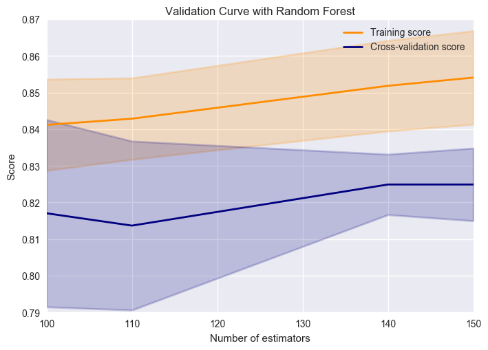
from sklearn.model_selection import validation_curve
X, y = X_train,Y_train['Survived']
#X, y = train_new,Y_train['Survived']
def cross_val(model,X,y,pname):
param_range = np.array([100,110,140,150])
train_scores, test_scores = validation_curve(
model, X, y, param_name=pname, param_range=param_range, scoring="accuracy", n_jobs=4)
train_scores_mean = np.mean(train_scores, axis=1)
train_scores_std = np.std(train_scores, axis=1)
test_scores_mean = np.mean(test_scores, axis=1)
test_scores_std = np.std(test_scores, axis=1)
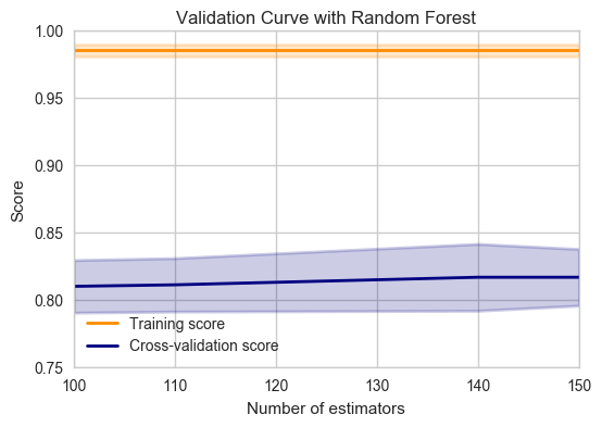
plt.title("Validation Curve with Random Forest")
plt.xlabel("Number of estimators")
plt.ylabel("Score")
lw = 2
plt.plot(param_range, train_scores_mean, label="Training score",
color="darkorange", lw=lw)
plt.fill_between(param_range, train_scores_mean - train_scores_std,
train_scores_mean + train_scores_std, alpha=0.2,
color="darkorange", lw=lw)
plt.plot(param_range, test_scores_mean, label="Cross-validation score",
color="navy", lw=lw)
plt.fill_between(param_range, test_scores_mean - test_scores_std,
test_scores_mean + test_scores_std, alpha=0.2,
color="navy", lw=lw)
plt.legend(loc="best")
plt.show()
cross_val(RandomForestClassifier(),X,y,'n_estimators')
from sklearn.model_selection import learning_curve
from sklearn.model_selection import ShuffleSplit
def plot_learning_curve(estimator, title, X, y, ylim=None, cv=None,
n_jobs=1, train_sizes=np.linspace(.1, 1.0, 5)):
"""
Generate a simple plot of the test and training learning curve.
Parameters
----------
estimator : object type that implements the "fit" and "predict" methods
An object of that type which is cloned for each validation.
title : string
Title for the chart.
X : array-like, shape (n_samples, n_features)
Training vector, where n_samples is the number of samples and
n_features is the number of features.
y : array-like, shape (n_samples) or (n_samples, n_features), optional
Target relative to X for classification or regression;
None for unsupervised learning.
ylim : tuple, shape (ymin, ymax), optional
Defines minimum and maximum yvalues plotted.
cv : int, cross-validation generator or an iterable, optional
Determines the cross-validation splitting strategy.
Possible inputs for cv are:
- None, to use the default 3-fold cross-validation,
- integer, to specify the number of folds.
- An object to be used as a cross-validation generator.
- An iterable yielding train/test splits.
For integer/None inputs, if ``y`` is binary or multiclass,
:class:`StratifiedKFold` used. If the estimator is not a classifier
or if ``y`` is neither binary nor multiclass, :class:`KFold` is used.
Refer :ref:`User Guide <cross_validation>` for the various
cross-validators that can be used here.
n_jobs : integer, optional
Number of jobs to run in parallel (default 1).
"""
plt.figure()
plt.title(title)
if ylim is not None:
plt.ylim(*ylim)
plt.xlabel("Training examples")
plt.ylabel("Score")
train_sizes, train_scores, test_scores = learning_curve(
estimator, X, y, cv=cv, n_jobs=n_jobs, train_sizes=train_sizes)
train_scores_mean = np.mean(train_scores, axis=1)
train_scores_std = np.std(train_scores, axis=1)
test_scores_mean = np.mean(test_scores, axis=1)
test_scores_std = np.std(test_scores, axis=1)
plt.grid()
plt.fill_between(train_sizes, train_scores_mean - train_scores_std,
train_scores_mean + train_scores_std, alpha=0.1,
color="r")
plt.fill_between(train_sizes, test_scores_mean - test_scores_std,
test_scores_mean + test_scores_std, alpha=0.1, color="g")
plt.plot(train_sizes, train_scores_mean, 'o-', color="r",
label="Training score")
plt.plot(train_sizes, test_scores_mean, 'o-', color="g",
label="Cross-validation score")
plt.legend(loc="best")
return plt
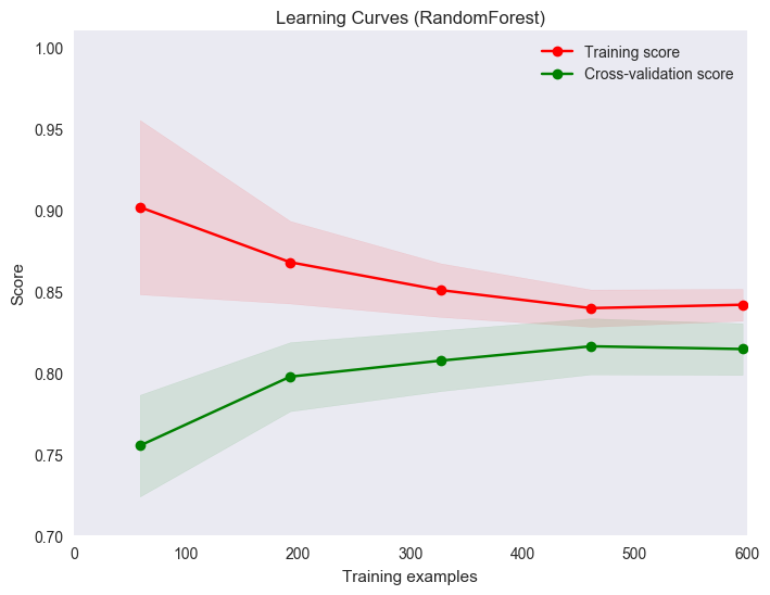
title = "Learning Curves (RandomForest)"
# Cross validation with 100 iterations to get smoother mean test and train
# score curves, each time with 20% data randomly selected as a validation set.
#cv = ShuffleSplit(n_splits=20, test_size=0.33, random_state=0)
#estimator=RandomForestClassifier(n_estimators=100)
#plot_learning_curve(estimator, title, X, y, ylim=(0.7, 1.01), cv=cv, n_jobs=4)
Hmm, underfitting :/
The prediction seems good enough for now, let’s submit’…
… Or maybe not. First public submission got 0.65. Time to try another method?
About 0.775 with RandomForests. One final trial, with XGBoost
from xgboost import XGBClassifier
from sklearn.metrics import accuracy_score
from sklearn.model_selection import StratifiedKFold
from sklearn.model_selection import GridSearchCV
# fit model no training data
model = XGBClassifier()
model_params = {
    'learning_rate': [0.05, 0.1],
    'n_estimators': [100,150,200],
    'max_depth': [2, 3,7, 10],
}
cv = StratifiedKFold()
cv.get_n_splits(X_train,Y_train)
grid= GridSearchCV(model,model_params,scoring='roc_auc',cv=cv,verbose=2)
best_params={'n_estimators': 100, 'max_depth': 2, 'learning_rate': 0.05}
#grid.fit(X_train, Y_train.values.ravel())
model = XGBClassifier(n_estimators= 100, max_depth= 2, learning_rate= 0.05)
model.fit(X_train,Y_train.values.ravel())

# Take the same decision trees and run it on the test data
Y_pred = model.predict(X_test)
#Y_pred = [round(value) for value in Y_pred]
#cross_val(XGBClassifier(),X,y,'n_estimators')
#About 200 seems okay
title = "Learning Curves (RandomForest)"
# Cross validation with 100 iterations to get smoother mean test and train
# score curves, each time with 20% data randomly selected as a validation set.
cv = ShuffleSplit(n_splits=10, test_size=0.33, random_state=0)
mpl.rcParams['figure.figsize'] = [8.0, 6.0]

plot_learning_curve(model, title, X, y, ylim=(0.7, 1.01), cv=cv)
<module 'matplotlib.pyplot' from '/home/artir/anaconda3/lib/python3.5/site-packages/matplotlib/pyplot.py'>
import matplotlib as mpl
sns.set()
cross_val(model,X,y,'n_estimators')
test.head()
| Pclass | Sex | Age | SibSp | Parch | Fare | Embarked | male | Class_1 | Class_2 | Class_3 | FamilySize | HaveFamily | child | |
|---|---|---|---|---|---|---|---|---|---|---|---|---|---|---|
| 0 | 3 | male | 34.5 | 0 | 0 | 7.8292 | Q | 1 | 0 | 0 | 1 | 0 | 0 | 0 |
| 1 | 3 | female | 47.0 | 1 | 0 | 7.0000 | S | 0 | 0 | 0 | 1 | 1 | 1 | 0 |
| 2 | 2 | male | 62.0 | 0 | 0 | 9.6875 | Q | 1 | 0 | 1 | 0 | 0 | 0 | 0 |
| 3 | 3 | male | 27.0 | 0 | 0 | 8.6625 | S | 1 | 0 | 0 | 1 | 0 | 0 | 0 |
| 4 | 3 | female | 22.0 | 1 | 1 | 12.2875 | S | 0 | 0 | 0 | 1 | 2 | 1 | 0 |
submission = pd.DataFrame({
        "PassengerId": test_df["PassengerId"],
        "Survived": Y_pred
    })
submission.to_csv('titanic.csv', index=False)
import sys
print(sys.version)
3.5.2 |Anaconda custom (64-bit)| (default, Jul  2 2016, 17:53:06)
[GCC 4.4.7 20120313 (Red Hat 4.4.7-1)]
Lessons learned
- Establishing a process for analysing the data is important, even if that process requires iteration
- It really comes down to explore the data, generate features, then feed to the algorithm
- Which algorithm? Apparently XGBoost is the best. Also, try neural nets with keras.
- Correlation plots are interesting to heuristically decide what to keep/drop. In the end
- Some plots are better than others, depending on the case